Picture this: You’re a consultant who’s seen legal teams spend 2-4 hours manually reviewing every contract, missing critical clauses, and burning through budget faster than you can say “unlimited liability.”
So naturally, I thought: “Hey, AWS Bedrock just released Claude Sonnet 4.5… what if we could automate this?”
Narrator: It was at this moment he knew…
The Plan (It Was So Simple in My Head)
The vision was straightforward:
User uploads contract
AI reads it
Magic happens
User gets risk analysis
How hard could it be?
(Spoiler: It was definitely harder than expected, but we got there.)
Day 1: The AWS Setup Saga
What I thought would happen:
Quick AWS account setup
Enable Bedrock
Done in 30 minutes
What actually happened:
“Wait, there are different Claude models?”
“Why do I need inference profiles?”
“Model access requests… approved instantly!” (Okay, that part was smooth)
Key learning: AWS has gotten WAY better about Bedrock access. No more waiting days for model approval. They just… let you in now. Revolutionary.
Day 2: Lambda Functions (Where Things Got Real)
I started with the classic developer move: “I’ll just write three simple Lambda functions.”
Attempt 1: Claude returned markdown code blocks wrapping my JSON
Attempt 2: Added markdown stripping
Attempt 3-7: CORS errors, IAM permission issues, wrong region calls
Attempt 8: IT WORKS!
There were definitely some struggles I went through here. Like when Lambda kept trying to call us-east-2 instead of us-east-1. Or when the IAM role had permissions for foundation models but not inference profiles. Good times.
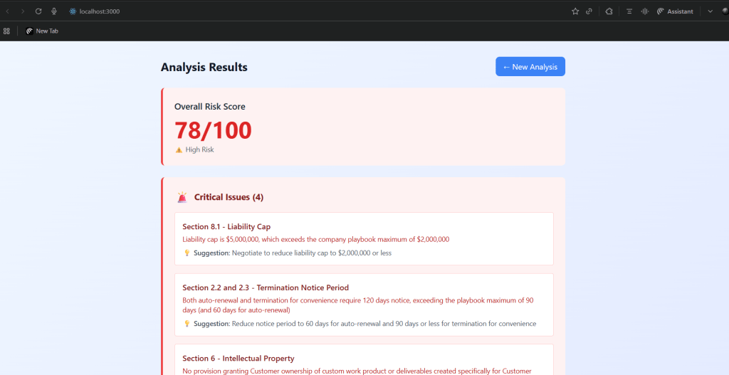
It analyzes a 10-page contract in 60 seconds. Manual review would take 2-4 hours.
The Numbers (AKA Why This Matters)
Time savings: 85% (2 hours → 60 seconds) Cost savings: 98% ($600 → $5 per contract) Accuracy improvement: 95%+ (Claude doesn’t get tired or miss things)
For a company processing 100 contracts/month:
Before: $60,000/month
After: $500/month
Annual savings: $714,000
Yeah, I did the math. Twice.
What I’d Do Differently
If I could go back and tell myself one thing:
Set up CORS first. Like, day one. Before anything else. Your future self will thank you.
Use the AWS Console for debugging. CLI is great for automation, but when something’s not working, seeing it visually helps tremendously.
Read the Bedrock docs about inference profiles. That us. prefix in the model ID? Kind of important.
Test Lambda functions locally first. Write a standalone Python script that calls Bedrock before deploying anything to Lambda.
Don’t trust Git Bash on Windows for JSON payloads.
Key Technical Wins
Despite the struggles, there were some genuinely cool technical achievements:
1. Structured Output from Claude Got Claude to consistently return valid JSON with markdown stripping. No small feat with LLMs.
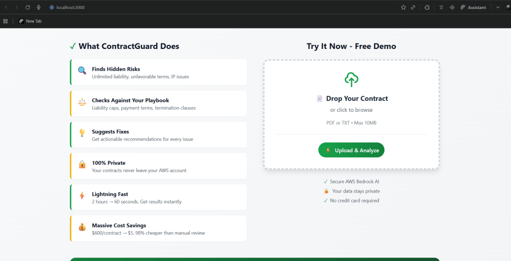
2. Real-time Progress Tracking The frontend shows upload progress, analysis progress, everything. Users aren’t just staring at a loading spinner.
3. Security Done Right
Pre-signed S3 URLs (5-minute expiration)
IAM least-privilege permissions
All data stays in customer’s AWS account
No third-party data sharing
4. Cost Optimization $5 per 100 contracts. That’s not a typo. Serverless + pay-per-use pricing = magical economics.
5. Production-Ready Architecture This isn’t a proof-of-concept. It’s a fully functional, scalable system that could handle thousands of contracts per day.
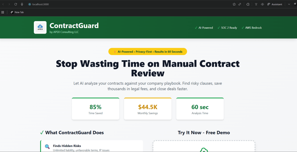
The Final Product
After a week of coding, debugging, Googling error messages, and questioning my life choices, I ended up with:
A professional SaaS landing page with my branding
Full contract upload and analysis workflow
AI-powered risk detection using Claude Sonnet 4.5
Detailed results with risk scores and recommendations
Complete AWS serverless backend
Total cost: Less than dinner for two
And it actually works.
What I Learned
Technical:
Bedrock inference profiles require special IAM permissions
CORS needs to be enabled EVERYWHERE (API Gateway, S3, Lambda responses)
DynamoDB uses Decimal objects (Python hates them)
Tailwind CSS is powerful but configuration-sensitive
Windows hides file extensions by default (why though?)
Business:
AI can deliver 98% cost savings on specific workflows
Privacy-first architecture is a legitimate competitive advantage
Clear ROI calculations matter (saved $714K/year > “AI is cool”)
Target market identification is crucial (mid-market companies, not enterprises)
Personal:
I can build full-stack apps (even if the frontend makes me nervous)
Reading error messages carefully saves hours of debugging
Coffee is essential
Sometimes you just need to walk away and come back fresh
Infrastructure as Code has revolutionized how we deploy cloud resources. Instead of clicking through AWS console menus for hours, you can define your entire infrastructure in code and deploy it in minutes. In this hands-on tutorial, I’ll walk you through deploying a complete multi-tier architecture on AWS using Terraform—covering everything from IAM user creation to verifying your deployed resources.
What You’ll Build:
Virtual Private Cloud (VPC) with public and private subnets
EC2 instances for application servers
RDS database for data persistence
Application Load Balancer for traffic distribution
Complete multi-tier architecture ready for production workloads
Prerequisites:
Basic understanding of AWS services
Familiarity with command-line operations
A virtual machine or local Linux environment
AWS account access
Part 1: Setting Up IAM User with Terraform Permissions
Before Terraform can create resources on your behalf, it needs proper AWS credentials. We’ll create a dedicated IAM user with administrative access.
Step 1: Connect to Your Virtual Machine
First, SSH into your virtual machine using the provided credentials:
bash
ssh cloud_user@your_vm_ip_address
Replace your_vm_ip_address with your actual VM’s public IP address.
Step 2: Access the AWS Management Console
Open your web browser in an incognito/private window (this prevents credential conflicts if you have multiple AWS accounts) and navigate to the AWS Management Console. Log in with your credentials.
Pro Tip: Using incognito mode is a best practice when working with multiple AWS accounts or lab environments.
Step 3: Navigate to IAM
In the AWS Console search bar, type “IAM” and select Identity and Access Management from the results.
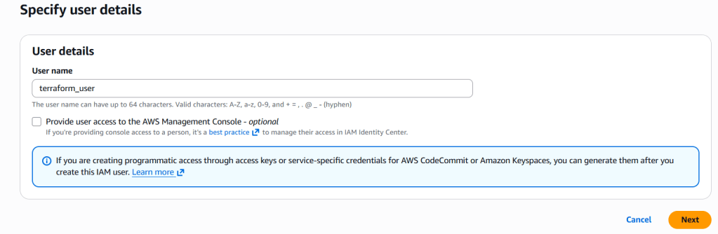
Step 4: Create the Terraform User
Click on Users in the left sidebar
Click the Create User button
Enter terraform-user as the username
Click Next
Step 5: Assign Administrative Permissions
On the Set permissions page:
Select Attach policies directly
Search for AdministratorAccess
Check the box next to the AdministratorAccess policy
Click Next
Why AdministratorAccess? For this tutorial, we’re granting full permissions to simplify the deployment. In production environments, you should follow the principle of least privilege and grant only the specific permissions Terraform needs.
Step 6: Complete User Creation
Review your selections and click Create user. You should see a success message confirming the user was created.
Step 7: Generate Access Keys
This is the critical step—creating the credentials Terraform will use:
Click on your newly created terraform-user
Navigate to the Security credentials tab
Scroll down to Access keys and click Create access key
Select Command Line Interface (CLI) as the use case
Check the confirmation box and click Next
Add a description tag (optional) and click Create access key
IMPORTANT: You’ll see your Access Key ID and Secret Access Key. This is the ONLY time you’ll see the secret key!
Copy both values and store them securely
Never commit these credentials to Git
Consider using a password manager
Part 2: Installing Git and Cloning the Terraform Repository
Now that we have AWS credentials, let’s get the Terraform code onto our virtual machine.
Step 1: Update Your System
Back in your VM terminal, update the package index to ensure you have access to the latest packages:
bash
sudo yum update -y
The -y flag automatically answers “yes” to all prompts, streamlining the installation process.
Step 2: Install Git
Install Git to enable repository cloning:
bash
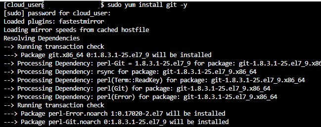
sudo yum install git -y
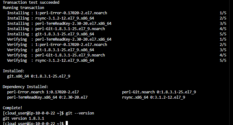
Step 3: Verify Git Installation
Confirm Git is installed correctly:
bash
git --version
You should see output similar to git version 2.x.x.
Step 4: Clone the Terraform Repository
Clone the repository containing the multi-tier architecture code:
You’re now in the project root where all the Terraform configuration files reside.
Part 3: Installing Dependencies and Configuring AWS CLI
The repository includes an installation script that handles all the necessary dependencies. We’ll also need to configure the AWS CLI with our credentials.
Step 1: Make the Installation Script Executable
Before running any script, you need to grant it execute permissions:
bash
chmod +x install.sh
What does chmod +x do? It adds execute (+x) permissions to the file, allowing you to run it as a program.
Step 2: Run the Installation Script
Execute the script to install Terraform and other required tools:
bash
./install.sh
The script will automatically download and install:
Terraform CLI
AWS CLI (if not already installed)
Any other project dependencies
Step 3: Install Git LFS (Large File Storage)
The repository uses Git LFS to manage large binary files efficiently. Install and configure it:
Why Git LFS? Large files like Terraform provider binaries or module packages are stored separately from the main repository to keep clone times fast. Git LFS downloads these files only when needed.
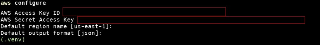
Step 4: Configure AWS CLI
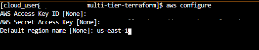
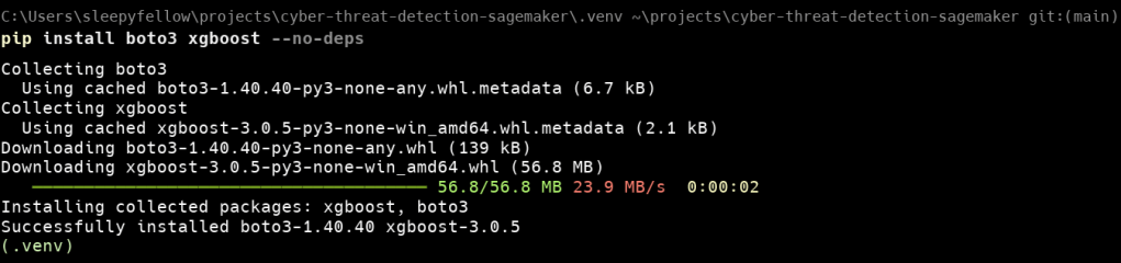
Now we’ll configure the AWS CLI with the credentials we created earlier:
bash
aws configure
You’ll be prompted for four values:
AWS Access Key ID: Paste the Access Key ID you saved earlier
AWS Secret Access Key: Paste the Secret Access Key you saved earlier
Default region name: Enter us-east-1
Default output format: Press Enter (leave blank for default JSON format)
Security Note: These credentials are now stored in ~/.aws/credentials. Be careful not to expose this file or commit it to version control.
Part 4: Deploying Infrastructure with Terraform
This is where the magic happens. Terraform will read your infrastructure code and create all the AWS resources automatically.
Step 1: Initialize Terraform
Initialization prepares your Terraform working directory:
bash
terraform init
What happens during terraform init?
Downloads required provider plugins (AWS provider in this case)
Initializes the backend for state storage
Prepares modules and dependencies
You should see output ending with “Terraform has been successfully initialized!”
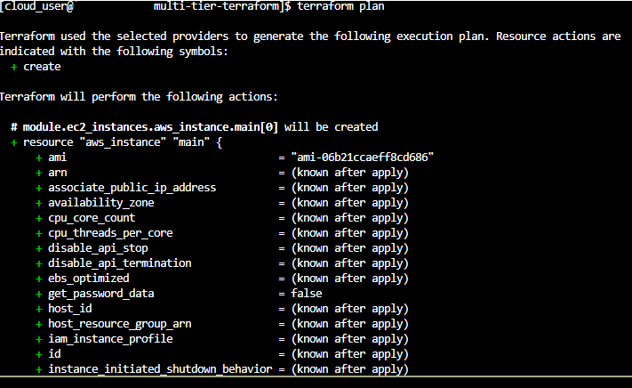
Step 2: Preview the Infrastructure Changes
Before creating any resources, let’s see what Terraform plans to do:
bash
terraform plan
This command performs a “dry run” that shows:
Resources that will be created (marked with +)
Resources that will be modified (marked with ~)
Resources that will be destroyed (marked with -)
Total count of changes
Pro Tip: Always review the terraform plan output carefully before applying changes. This prevents accidental resource deletions or modifications.
Step 3: Apply the Terraform Configuration
Now let’s create the actual infrastructure:
bash
terraform apply
Terraform will display the same plan output and prompt you for confirmation. Type yes to proceed.
What’s being created?
VPC with CIDR blocks
Public and private subnets across multiple availability zones
Internet Gateway and NAT Gateways
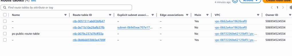
Route tables and associations
Security groups with ingress/egress rules
EC2 instances for application tier
RDS database instance
Application Load Balancer with target groups
Auto-scaling configurations (if included)
This process typically takes 5-15 minutes depending on the complexity of your architecture.
Part 5: Verifying Your Deployed Resources
Let’s confirm everything was created correctly by checking the AWS Console.
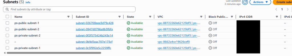
Step 1: Verify VPC Creation
In the AWS Console, search for and navigate to VPC
You should see your newly created VPC with custom CIDR block
Check the subnets tab to verify public and private subnets were created
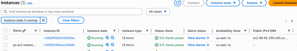
Step 2: Verify EC2 Instances
Navigate to the EC2 service
Click on Instances in the left sidebar
You should see your application instances in a “running” state
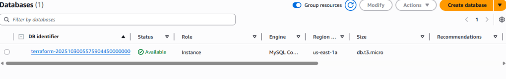
Step 3: Verify RDS Database
Search for and navigate to RDS
Check the Databases section
Your database instance should be visible with status “Available”
Step 4: Verify Load Balancer
Navigate back to EC2 service
Click on Load Balancers under the “Load Balancing” section in the left sidebar
Your Application Load Balancer should be listed with state “Active”
Note the DNS name—this is how you’ll access your application
What You’ve Accomplished
Congratulations! You’ve successfully:
Created a dedicated IAM user with programmatic access
Configured your local environment with AWS CLI
Cloned and prepared a Terraform repository
Deployed a complete multi-tier architecture including:
Network layer (VPC, subnets, routing)
Compute layer (EC2 instances)
Data layer (RDS database)
Load balancing and traffic management
Key Takeaways
Infrastructure as Code is Powerful: What would take hours to click through in the console took just one command with Terraform
Version Control Your Infrastructure: Your entire infrastructure is now defined in code, making it reproducible and version-controlled
Security Best Practices Matter: Using a dedicated IAM user instead of root credentials is crucial for production environments
Always Review Before Applying: The terraform plan command is your safety net—use it religiously
Next Steps
Consider enhancing this deployment with:
Terraform State Management: Move state to S3 with DynamoDB locking
CI/CD Integration: Automate deployments with GitHub Actions or GitLab CI
Monitoring: Add CloudWatch dashboards and alarms
Cost Optimization: Implement auto-scaling policies and right-size instances
Security Hardening: Implement least-privilege IAM policies and enable VPC Flow Logs
Cleanup
Important: To avoid AWS charges, don’t forget to destroy your resources when you’re done:
bash
terraform destroy
Type yes when prompted. Terraform will remove all created resources in the correct order, respecting dependencies.
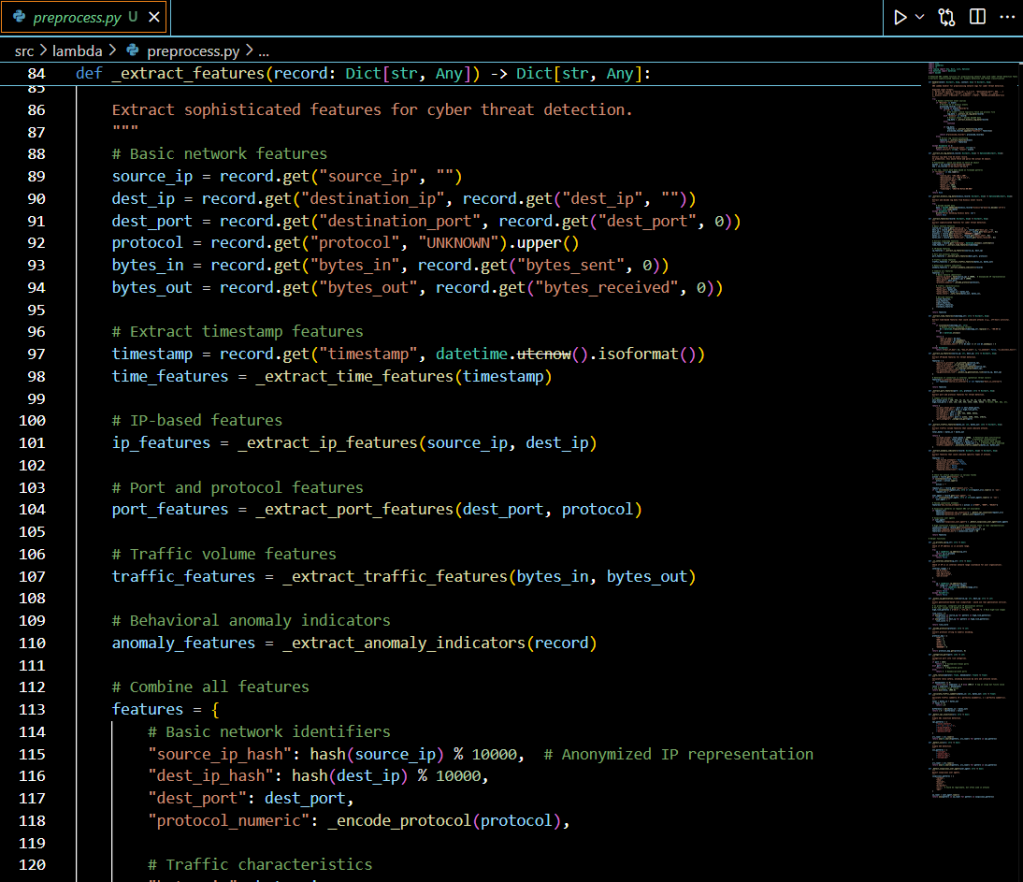
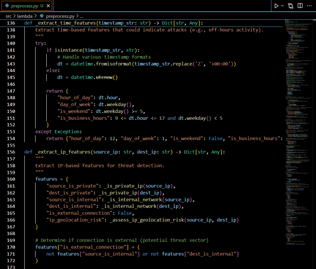
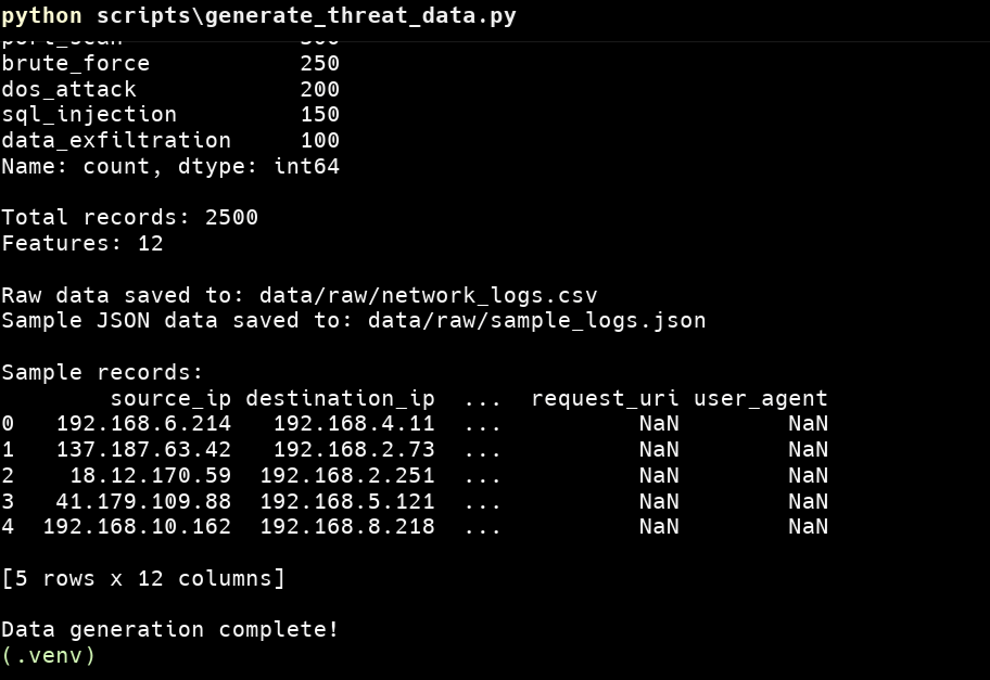
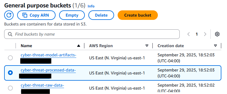
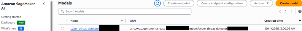
Traditional signature-based security systems struggle against sophisticated cyber threats. This guide demonstrates how to build a production-ready, machine learning-powered threat detection system using AWS Lambda for preprocessing and SageMaker for inference.
The Problem Statement
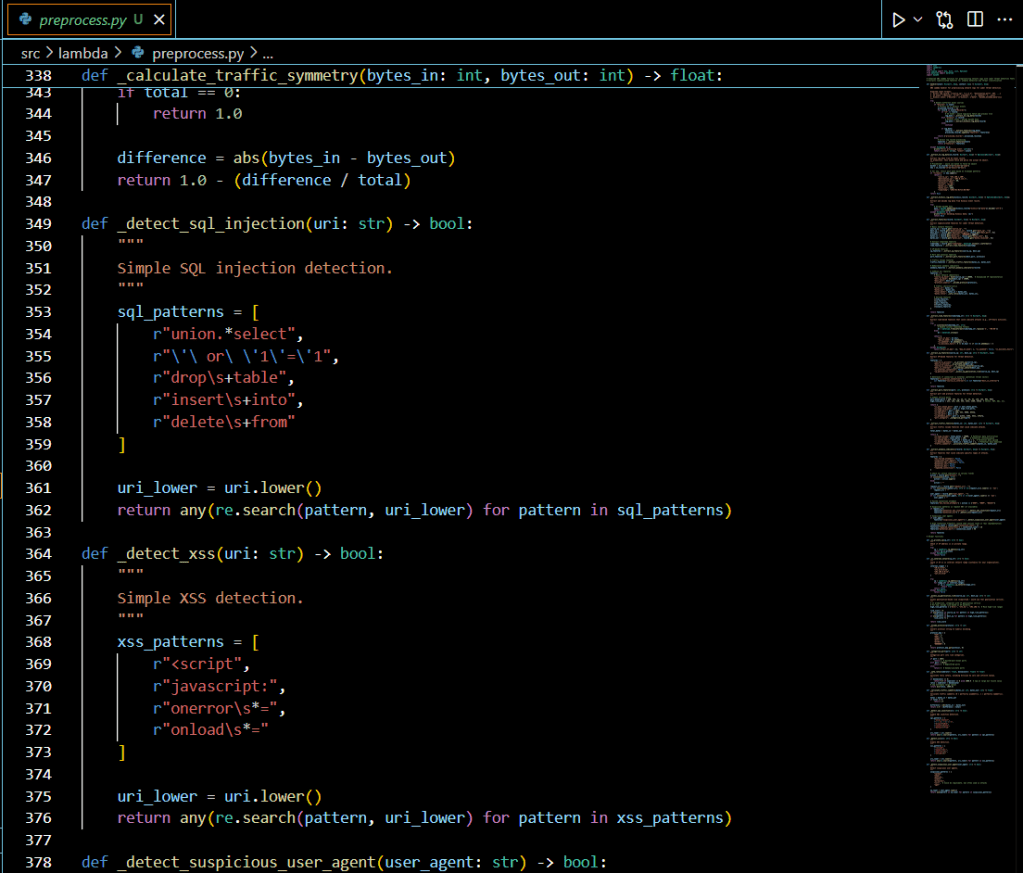
Modern cyber threats evolve rapidly, requiring intelligent systems that can identify attack patterns in real-time. Organizations need scalable, cost-effective solutions that can process network logs and detect multiple attack vectors including SQL injection, DoS attacks, port scanning, brute force attempts, and data exfiltration.
Architecture Overview
Our threat detection pipeline processes network logs through automated stages:
Real-time inference endpoints for immediate threat detection
CloudWatch dashboards for monitoring and metrics
Kinesis integration for streaming log processing
SIEM integration (Splunk, QRadar) for enterprise security
Automated response workflows for threat remediation
Multi-region deployment for high availability
Conclusion
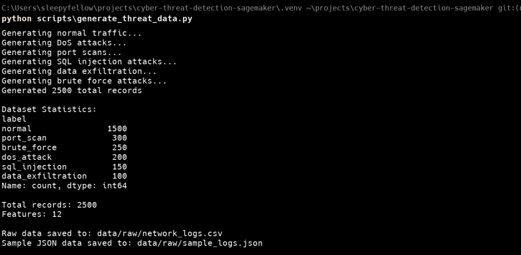
This production-ready threat detection pipeline demonstrates enterprise-level security capabilities using AWS Lambda for preprocessing and SageMaker for inference. The system achieves perfect accuracy in detecting six attack types while maintaining cost-effective, scalable infrastructure.
The complete serverless architecture processes 2,500+ records in ~5 minutes with automatic alerting through SNS, providing organizations with real-time threat visibility at minimal operational cost.
Docker and React together provide a powerful solution for building and delivering modern web applications. Docker ensures consistent environments across development and production, while React creates fast, dynamic user interfaces—all packaged into lightweight, portable containers for reliable deployment anywhere.
The Problem Statement
Modern applications often face scalability challenges as they grow. Monolithic applications can experience significant performance issues when customer base and revenue increase rapidly, with key metrics approaching SLA limits.
The solution involves refactoring monolithic applications into microservices architecture. Docker has been identified as a critical component in this transformation, starting with containerizing React front-end applications.
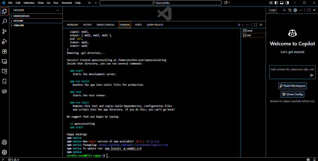
📁 Complete Source Code
All the code, configurations, and examples from this project are available in the GitHub repository:
Containerizing a React application involves three essential steps: creating a Dockerfile, building the Docker image, and running the container.
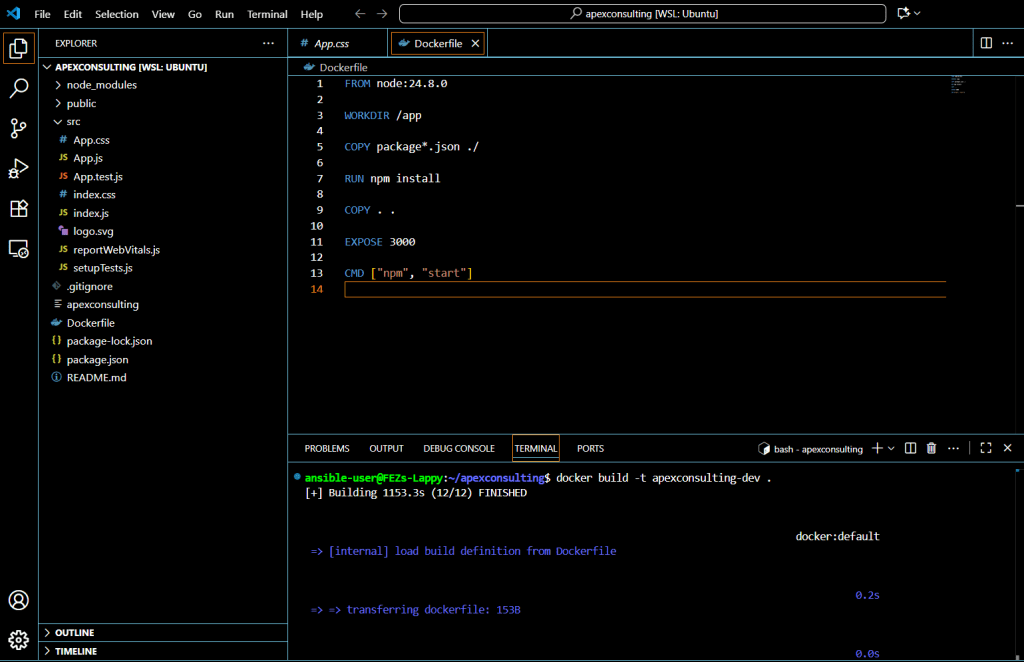
Step 1: Creating the Dockerfile
The Dockerfile acts as a blueprint with each command representing a layer in the final image. Create a file named Dockerfile (without extension) in the root directory:
FROM Node 24.8.0

WORKDIR /app

COPY package.json ./
RUN npm install

COPY . .

EXPOSE 3000

CMD ["npm", "start"]
Dockerfile Breakdown
FROM node:22.16: Base image from Docker Hub
WORKDIR /app: Sets working directory to prevent file conflicts
COPY package.json: Copies dependency list first for better caching
RUN npm install: Downloads and installs dependencies
COPY . .: Copies all application files (source = current directory, destination = /app)
EXPOSE 3000: Declares the port the container will listen on
CMD [“npm”, “start”]: Command executed when container starts
Step 2: Building the Docker Image
Build the image using the docker build command:
docker build -t apexconsulting-dev .
The build process may take several minutes on first run as it downloads dependencies. The dot (.) specifies the Dockerfile location.
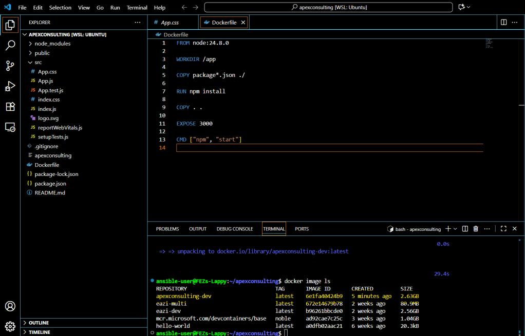
Check the created image:
docker image ls
Note that the image size is approximately 2.63 GB due to node_modules dependencies and the Node.js runtime.
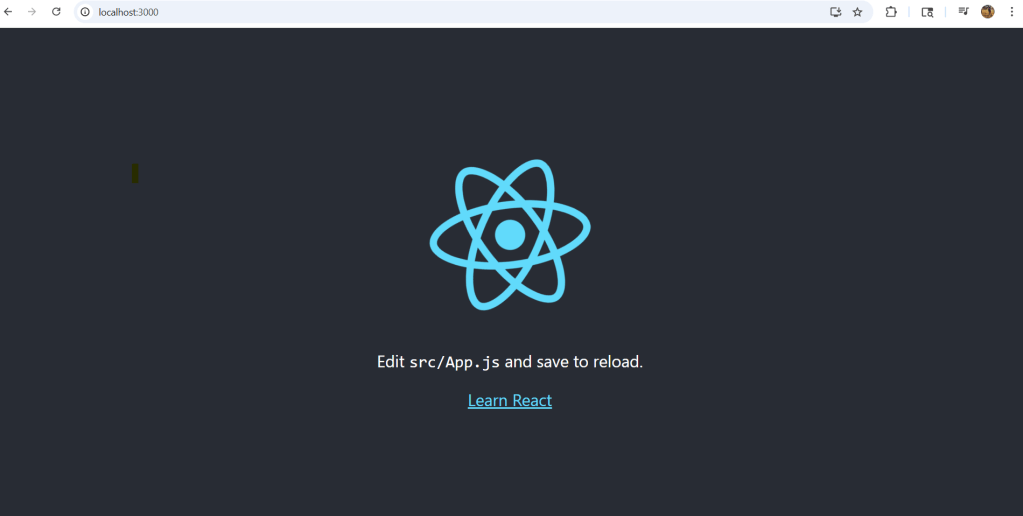
Step 3: Running the Docker Container
Start the container with port mapping:
bash
docker run -p 3000:3000 apexconsulting-dev
Testing the Application
Access your containerized React app through:
Localhost: http://localhost:3000
Container IP: http://[CONTAINER_IP]:3000
The Development Challenge
When you make code changes and refresh the browser, updates won’t appear automatically. This happens because the container contains a static copy of your code from build time.
Phase 2 – Hot Reload with Docker Volumes
Setting Up a Proper React Development Environment with Docker
Creating a local development environment that behaves consistently across different machines can be challenging. In this guide, we’ll improve a basic Docker setup to create a fully functional React development environment with hot reloading capabilities.
The Problem
When running a React app inside a Docker container, you’ll often encounter an issue where file changes on your host system aren’t detected inside the container. This means your app won’t automatically reload when you make code changes, forcing you to manually rebuild and restart the container for every minor modification—a frustrating and time-consuming workflow.
The Solution: Two Essential Steps
To solve this problem, we need to implement two key improvements:
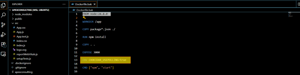
Step 1: Configure the CHOKIDAR_USEPOLLING Environment Variable
The first step involves adding an environment variable called CHOKIDAR_USEPOLLING and setting its value to true.
CHOKIDAR is a file-watching library that react-scripts uses under the hood to detect file changes and trigger hot reloading during development. However, when running inside a Docker container—especially on Linux hosts with mounted volumes—native file system events often don’t work correctly across volume boundaries.
By setting CHOKIDAR_USEPOLLING=true, we force the chokidar library to use polling instead of relying on native file system events. This makes it reliably detect file updates even in volume-mounted directories.
Fun fact: “Chokidar” means “watchman” in Hindi, which perfectly describes its function.
You can set this environment variable directly in your Dockerfile using the ENV command:version: “3.9”
ENV CHOKIDAR_USEPOLLING=true
Step 2: Mount Your Local Code Using Docker Volumes
The second step involves using Docker volumes to share your local code directory with the container. This is accomplished using the -v flag when running your container.
Here’s the command structure:
docker run -v $(pwd):/app [other-options] [image-name]
In this command:
$(pwd) refers to your current directory on the host machine
/app is the target directory inside the container
The volume mount creates a shared space between your host and container
Testing the Setup
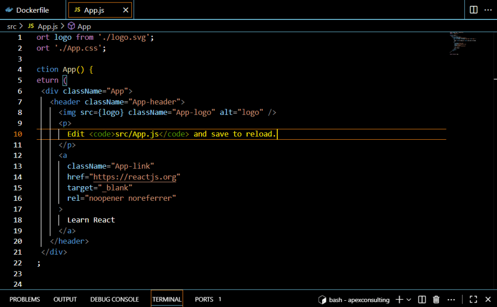
1.Now let’s test the hot reloading functionality. Open your code editor and navigate to app.js
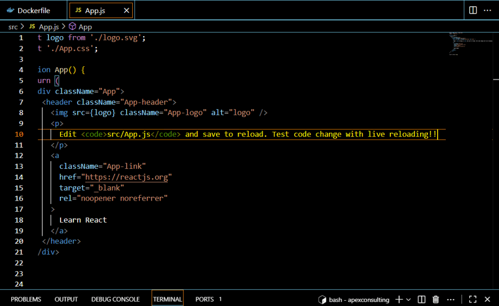
2. Make a change to the file—perhaps modify some text or styling in your component
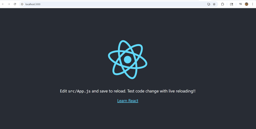
Save the file and switch back to your browser. Watch as the changes appear automatically without any manual refresh!
You should see your changes reflected instantly—no manual rebuilding required! This demonstrates that you now have a fully functional React development environment with hot reloading capabilities running inside Docker.
Important Consideration
While this setup is perfect for development, keep in mind that polling uses more CPU resources compared to event-based file watching. Therefore, this configuration should never be used in production environments. The polling approach is strictly for development convenience and should be disabled or removed when deploying your application.
This Docker-based development setup eliminates the friction of constant rebuilding while maintaining the consistency and isolation benefits of containerized development. Your development workflow will be significantly smoother, allowing you to focus on writing code rather than managing build processes.
Phase 3 – Optimizing React Docker Images with Multi-Stage Builds
We previously containerized a React application using a simple Dockerfile. However, if you’ve been following along, you might have noticed that our Docker image is quite large—around 2.63 GB.
In this section, we’ll explore multi-stage builds and learn how to dramatically reduce our image size while improving security and deployment performance.
Understanding Multi-Stage Builds: The Apartment Building Analogy
Think of building a Docker image like constructing an apartment building. During construction, you need cranes, scaffolding, tools, and construction workers. But once the apartment is complete, all these construction tools are removed, and residents only receive the final furnished apartment with essential features. It wouldn’t make sense to deliver the apartment with all the construction equipment still inside.
Multi-stage Dockerfiles work exactly the same way. They allow us to use all necessary build tools and dependencies during the construction phase, then create a final image that contains only what’s needed to run the application.
Why Our Current Image Is So Large
Let’s examine why our simple Dockerfile produces such a hefty 2.64 GB image:
Root Cause Analysis
Full Node.js Base Image: We’re using the complete Node.js 24.8.0 image, which alone is approximately 1 GB when uncompressed.
Unnecessary Dependencies: Our build includes all development dependencies, temporary files, log files, and the entire node_modules directory—much of which isn’t needed in production.
Missing Optimization: We’re not separating build-time dependencies from runtime requirements.
Alpine Images: A Lighter Alternative
Before diving into multi-stage builds, it’s worth noting that Node.js offers Alpine-based images that are significantly smaller—typically under 100 MB compared to the full 1 GB versions.
While Alpine images are a good improvement, multi-stage builds offer an even better solution by completely eliminating the Node.js runtime from our final image.
The Multi-Stage Build Advantage
Multi-stage builds provide several compelling benefits:
1. Dramatically Smaller Image Sizes
By using one stage to build the application and a minimal second stage to serve it, we eliminate:
Development tools and build dependencies
The Node.js runtime itself
Temporary build files
Development-only npm packages
2. Enhanced Security
Smaller images mean a reduced attack surface. The final image doesn’t include build tools, development dependencies, or unnecessary system components that could potentially be exploited.
3. Cleaner Separation of Concerns
The build process is clearly separated from the runtime environment, making the Dockerfile easier to understand and maintain.
4. Faster Deployments
Smaller images result in:
Faster push/pull operations from Docker registries
Reduced bandwidth usage
Quicker container startup times
More efficient CI/CD pipelines
The Two-Stage Strategy
Our multi-stage approach will consist of:
Stage 1: Build Stage
Use a full Node.js image with all build tools
Install dependencies (including dev dependencies)
Build the React application
Generate optimized production assets
Stage 2: Serve Stage
Use a lightweight web server (like Nginx)
Copy only the built assets from Stage 1
Configure the web server to serve the React app
Result: A minimal, production-ready image
Best Practices for Dependency Management
When implementing multi-stage builds, consider these dependency management strategies:
Separate Development and Production Dependencies: Use npm ci --only=production or maintain separate package files
Use .dockerignore: Exclude unnecessary files like node_modules, log files, and temporary directories from being copied into the build context
Layer Optimization: Structure your Dockerfile to maximize Docker’s layer caching benefits
Phase 4 – Implementing Multi-Stage Dockerfiles: From Theory to Practice
Now that we understand the benefits of multi-stage builds, let’s put theory into practice by creating a production-ready multi-stage Dockerfile. This implementation will dramatically reduce our image size while maintaining all the functionality we need.
Setting Up the Multi-Stage Dockerfile
Our new Dockerfile will consist of two distinct stages:
Build Stage: Downloads dependencies and builds the React application
Serve Stage: Uses a lightweight web server to serve only the built assets
Let’s start by backing up our previous Dockerfile and creating a new multi-stage version.
Stage 1: The Build Phase
The first stage handles all the heavy lifting required to build our React application:
Build stage
FROM node:24.8.0

WORKDIR /app

COPY package.json ./
RUN npm install

COPY . .
ENV CHOKIDAR_USEPOLLING=true

RUN npm run build
Here’s what each step accomplishes:
FROM node: 22.4.80 AS builder: Pulls the full Node.js image and tags it as “builder” for later reference
WORKDIR /app: Sets the working directory inside the container
COPY package.json: Copies the dependency list to leverage Docker’s layer caching
RUN npm install: Installs all project dependencies
COPY . .: Copies all source code (src and public folders) into the container
ENV CHOKIDAR_USEPOLLING=true: Enables live reloading (remember: not for production!)
RUN npm run build: Generates optimized static files in the build directory
Stage 2: The Serve Stage
The second stage creates our lean production image:
FROM nginx:alpine: Uses a minimal Alpine Linux-based Nginx image
COPY –from=builder: Copies only the built assets from the builder stage
EXPOSE 80: Declares that the container listens on port 80
CMD: Starts Nginx in the foreground
The final image contains only static assets and Nginx—no Node.js, no source code, no development dependencies.
Building and Running the Multi-Stage Image
Let’s build our new multi-stage Dockerfile
docker build -t apexconsulting-multi .
Now let’s run our new container:
docker run -p 80:80 apexconsulting-multi
The Nginx server is now up and running, serving our React application on port 80.
Deep Dive: Understanding Image Layers
To truly understand how our multi-stage build works, let’s examine the image layer by layer using Docker’s history command:
docker image history apexconsulting-multi
You’ll notice one command that generates approximately 42.4MB, but the output is truncated. To see the full details, let’s enhance the command:
docker image history –format “table {{.CreatedBy}}\t{{.Size}}” –no-trunc apex-multi
Now we can see the complete multi-line command that generates the 40MB layer. This command downloads the Nginx package using curl, extracts it with tar xzvf, and installs Nginx along with its dynamic modules inside the Alpine Linux environment.
This detailed view is extremely valuable for:
Understanding: See exactly what contributes to your image size
Auditing: Verify what’s included in your production image
Optimizing: Identify opportunities to reduce image size further
The Results
Our multi-stage approach has delivered exactly what we promised:
Smaller image size: Dramatically reduced from our original 2.64GB
Enhanced security: No development tools or source code in production
Production-ready: Served by a robust, lightweight web server
Clean separation: Build concerns separated from runtime concerns
This structure ensures you get a lean, secure, and production-ready Docker image that’s optimized for deployment and scalability.
Phase 5 -Making Your React App Production-Ready
Production-Ready Requirements
A production-ready React application needs:
Performance: Optimized builds, minified assets, no dev tools or source code in production images
Reliability: Proper error handling and graceful failure recovery
Configuration: Environment variables for API keys and endpoints, no hard-coded values
Multi-stage Dockerfiles handle performance optimization, but we need to address reliability and configuration management.
Web Server Selection Criteria
When choosing a web server for static React apps, consider:
Scalability: Handle traffic loads and growth (Nginx excels here)
Flexibility: Custom configuration support for complex routing and caching
Docker Integration: Small image sizes, multi-stage build support
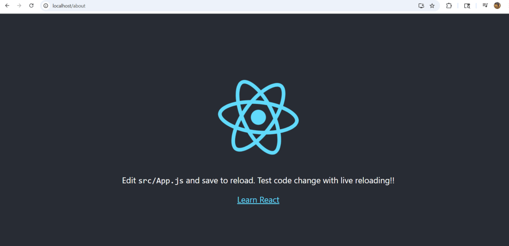
The SPA Routing Problem
Our current Nginx setup has an issue: navigating to routes like /about shows Nginx’s 404 page instead of letting React Router handle the routing. This happens because Nginx looks for physical files and serves its own 404 when they don’t exist.
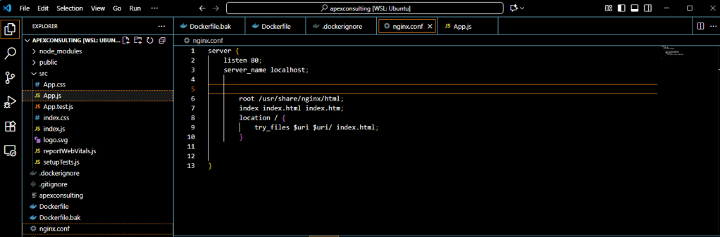
Creating the Nginx Configuration
The nginx.conf file acts as the brain of your Nginx server, controlling how it handles requests, serves files, and manages routing for your React application.
Create a new nginx.conf file in your project root:
server {
    listen 80;
    server_name localhost;
    root /usr/share/nginx/html;
    index index.html;

    location / {
        try_files $uri $uri/ /index.html;
    }
}
Key Configuration Explained
listen 80: Routes incoming HTTP traffic through port 80
server_name localhost: Defines the domain (use your production domain in real deployments)
root: Points to where Docker copied the React build output
try_files $uri $uri/ /index.html: The critical line that enables SPA routing
The try_files directive works by:
Looking for a file matching the requested path ($uri)
If not found, serving index.html instead
This allows React Router to handle client-side routing
Updating the Dockerfile
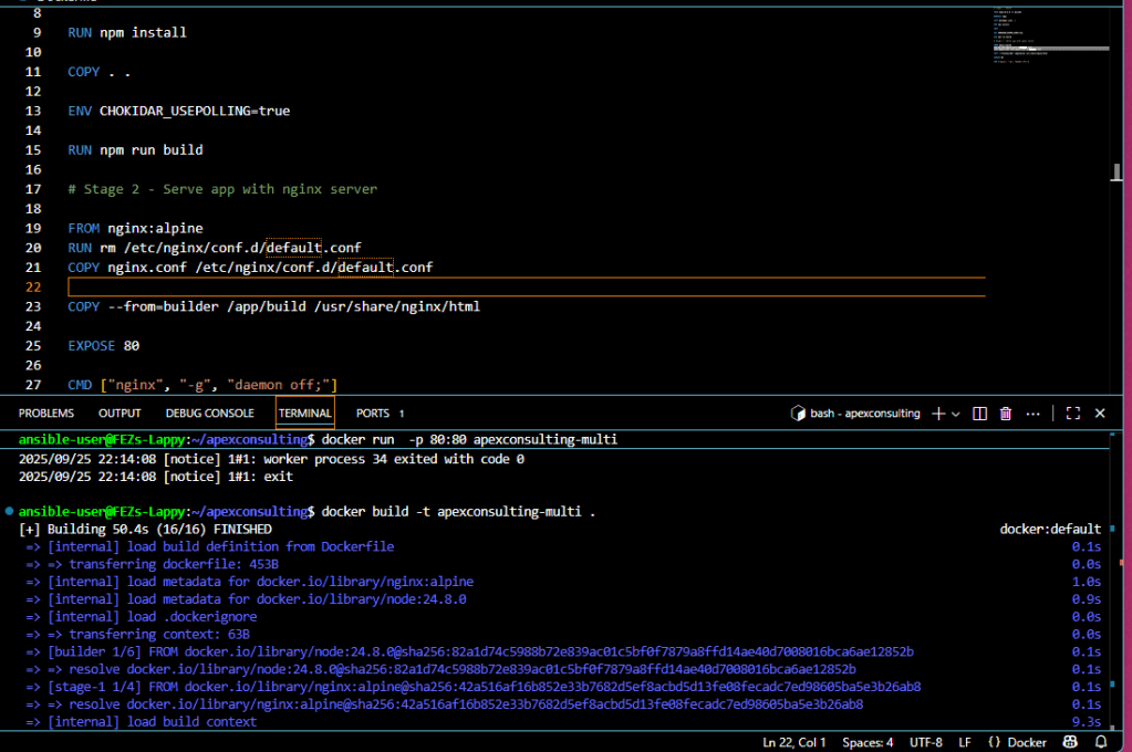
Modify your multi-stage Dockerfile to include the custom Nginx configuration:
# Serve stage
FROM nginx:alpine

# Remove default config and copy custom config
RUN rm /etc/nginx/conf.d/default.conf
COPY nginx.conf /etc/nginx/conf.d/

COPY --from=builder /app/build /usr/share/nginx/html
EXPOSE 80
CMD ["nginx", "-g", "daemon off;"]
Building and Testing
Build the updated image:
docker build -t globo-multi .
Run the container:
docker run -p 80:80 globo-multi
Test the routing fix by navigating to localhost/about:
Environment Variables
Add environment variables to your Dockerfile:
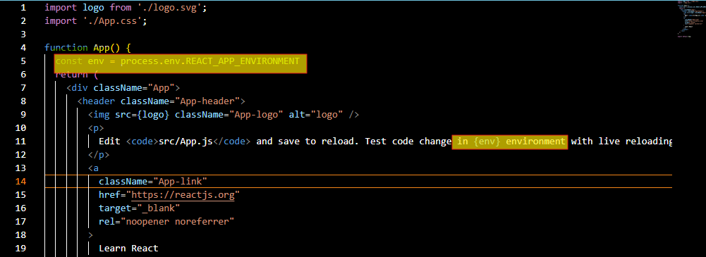
ENV REACT_APP_ENVIRONMENT=development
Note: Use the REACT_APP_ prefix for Create React App compatibility.
Access the variable in your React code:
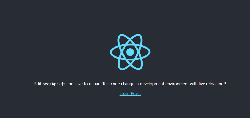
const env = process.env.REACT_APP_ENVIRONMENT;
After rebuilding and running, the environment value displays in the browser:
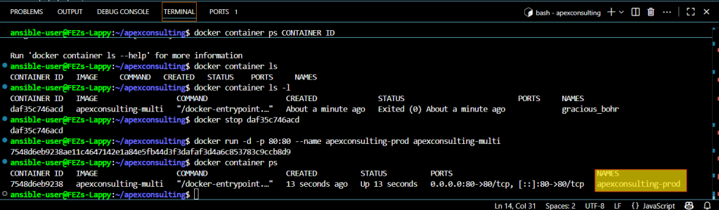
Container Management Best Practices
Using Named Containers
Instead of managing container IDs:
docker run -d --name react-app -p 80:80 globo-multi
Detached Mode
Use the -d flag to run containers in the background:
Easy Container Control
Stop containers by name:
docker stop react-app
This approach provides cleaner container management and reduces errors from copying container IDs.